↬ Analyze

Description

Survival statistics, or time-to-event studies, are commonly used in clinical trials, typically to observe the effect of intervention on disease progression. It follows participants throughout the time period of the study, recording their status ( i.e. whether their disease has progressed, or if death has occurred) in a binary fashion. This data can be represented as a “Kaplan-Meir plot” , which is useful for determining the prognosis of a disease and the efficacy of different treatments. The statistics used to obtain the results under the “groups” tab is similar to the statistics used in Cox proportional Hazards model.

Assumptions

1. Censored participants (those lost to follow up either part-way through the study, or because the study has ended) have the same likelihood of survival as those continuing in the study.
2. Survival probabilities are constant throughout, and the same for all participants - other survival statistics may incorporate fluctuating hazard, as time progresses. (known as proportional hazards function assumption)

Formatting

• Time - This is the time from when the participant joined, to the time of the event/end of the study/end of follow up. This is an important distinction, since participants may join at different points of the study, and may not all join at the start, or at the same time.
• Status - This is the column containing the status of each participant, at the given time. Typically it is specified as a binary event e.g. dead/alive, diagnosed/undiagnosed. For the statistics to be calculated, annotate the event within the status column as either a “1” or a “0” (i.e.. “1” = event has happened, and “0” = event has not happened). 
• Event - here you select the event that you wish to focus on, that is selected from the ‘status’ column (i.e. select whether to focus on “1” or “0”). 
• Group - this is the column that ascribes each participant to a group e.g. in an randomised control study, comparing an intervention vs a control group.

Worked Example

The downloadable example dataset follows a 14-month study examining two groups: ‘A’ and ‘B’, for the event of death (annotated in binary as “1”). The dataset is also separated into gender, under the column “sex” (1=female, 2= male)  This is a fabricated dataset, but it could be used to represent real life studies, for example; effect of Statins vs Placebo in reducing Coronary events, or the progression of an X-linked recessive disease.

Instructions

1. Download the example dataset
2. Click Analyze
3. Choose file type .xlsx
4. Browse for the file ‘Survival’
5. Select variables conveniently labelled ‘Time’, ‘Status’ and ‘Group’
6. Define Time as “Time”, Status as “Status”, and Group as “Group” or “Sex”
7. For the purposes of interpretation, Define Event as “1” (this performs statistics and plots graphs in concordance with the specified event)

Interpretation

Under the tab “Summary”, a brief summary is given, including the number of participants, number of events, and the proportion of events to N censored.

Under the tab “one group”, a summary of the survival statistics is given for the dataset, without segregating it into groups.

Under the tab “groups”, a summary of survival statistics is given for each specified group within the dataset. The area you should focus your attention on is given in the screenshot below. Below shows the output for group “sex”:

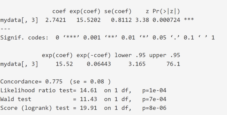
Z column - gives a metric of whether the coefficient of the variable being measured (in this instance it is sex) is significantly different from 0 (here it reads 3.38, with a signif.code of 0.05)

Sign under Coef -  (2.74) since it is positive, the higher the values of that variable, the worse the prognosis. Since sex is encoded as 1=female, and 2=male, being a male leads to a worse prognosis in this data.

Exp(coef) column - this gives the effect size of the variable. Here it reads 15.52. This is means that being male increases that hazard factor by around x15.5

Likelihood ratio, Wald Test and Score (log rank test) are all global measures of  significance of the model. If the P value is sufficiently low, then the findings of the comparison is said to be significant. Typically, their outputs are similar for large groups of N, although the outcome for the Likelihood ratio is generally preferred.

Under the tab ‘plot one’, a graph of “cumulative survival” against “time” is plotted. The survival curve decreases in its characteristic “step” fashion, which indicates the time at which an event has occurred. 

Under the tab ‘plot group’, The similar graph is plotted, except the participants are separated into their respective sex / grouping

Written by Kevin Michell

Resources

A nice, free introduction into Survival statistics https://www.ncbi.nlm.nih.gov/pmc/articles/PMC5045282/

↬ Analyze