


Normality of Distribution
Description
Distribution is a way of describing how data “looks”. Essentially, when plotted on a frequency distribution graph (Histogram), data will assume a certain “shape”, or distribution. By understanding what “shape” the data plot takes, it is possible to then make inferences about it. There are multiple types of data distribution, but this section will concentrate on a specific type called normal (or Gaussian/’Bell-shaped’) distribution. The purpose of this is to ensure the use of appropriate statistical analysis of the data as normal distribution and non-normal/parametric data require different tests.
Testing for normal distribution:
Normal distribution is the most common distribution found in nature. Tests such as the Student’s T-test or ANOVA, only work on normally distributed data. Hence, testing for normality, other than describing the data, can be a necessary first step before undertaking further statistical analysis.
Crudely, distribution can be tested by plotting the data on a histogram and seeing if its shape fits normal distribution. More precisely, however, mathematical tools can quantify how likely a set of data follows a normally distributed population. One such test is the Kolmogorov-Smirnov (KS) Test of Normality.
Kolmogorov-Smirnov (KS) Test:
This test mathematically compares your data to a normally distributed curve and quantifies the likelihood of your data being normally distributed. The test will generate the following results/values.
Test Statistic (D): How different your data is compared to a normal distribution (known as Divergence). The higher the value, the less likely it is that your data is normally distributed.
P-Value: Quantifies the probability that the divergence between your data and normal distribution is not caused by mere chance. The lower the P-value, the less likely your data is to be normally distributed.
Worked Example:
Download below example excel file 'Distribution'

- Click “Analyze” above
- Choose the file type (CVS or Excel)
- Upload your file
- Select “Height_(Cm)” as the variable
- Navigate the tabs on the right to find your results
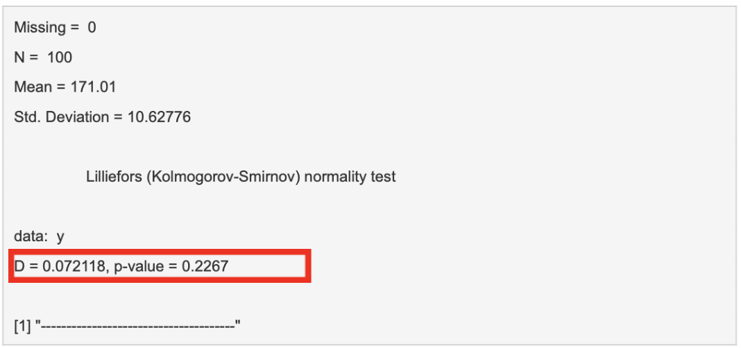
A low “D” value and a high p-value imply that there is no statistical difference between the distribution of our data and a normal distribution. We can therefore assume our data is normally distributed.
When selecting “Surgery_Number” as the variable, we obtain the below results:
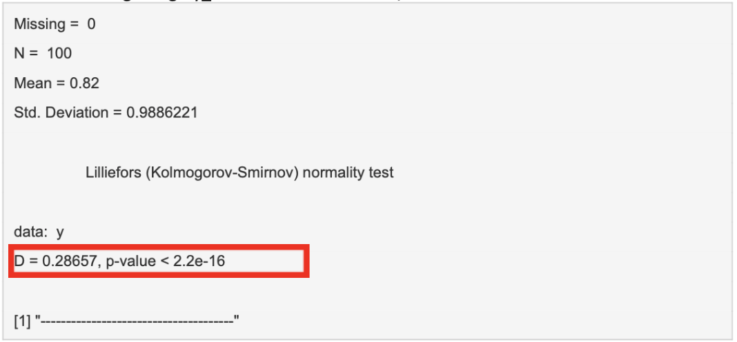
A high “D” value and a statistically significant p-value highlight the fact that there is a statistically significant difference between the distribution of our sample data and a normally distributed data set. We can therefore assume that this dataset is not normally distributed.
Written By Lorenzo Lenti